Saturday, January 29, 2011

Follow Up: More Graphics

I'm sticking these in a new post, rather than updating the last post (and potentially, nobody seeing them).


First of all, as I said yesterday, the 'entrance' squares of the snakes and ladders don't technically exist; in so much as, as soon as you land on them you move to the coresponding exit. So I updated the network graph to reflect this
But this version isn't quite as aesthetically pleasing as the other one. Still, at least no-one can accuse me of not doing it right.

And as you'd probably expect, the number of curves directed into a given square's node in the above graph is loosely related to the probability of visiting that square

And the other thing is, I wasn't happy with the board histogram - the bar chart of how often you land on each square. So I played with it a bit, to try and find the clearest, prettiest, and most easy to interpret representation of the data.

This is what I came up with
The numbers for entrances and exits are stacked, so you can see how often a given exit square is visited in total, and what proportion of those visits are from moving along a snake or ladder.

For example, there's about a 47% chance of getting to the end via the 80-100 ladder.

The arcs show which squares are linked.


Oatzy.

Friday, January 28, 2011

Snakes and Ladders

Or Chutes and Ladder, if you're American. Yes, I am talking about the board game.
The idea came from having read about people analysing Monopoly with simulations, Markov chains and the likes. You can read about it in Math Hysteria by Ian Stewart or find a similar discussion here.

In the book, Professor Stewart also suggests that the reader might like to try the same for Snakes and Ladders. So I did*.


If you're not familiar with Snakes and Ladders and how it works, you had a very deprived childhood. There's an example game board below
[wikipedia]

I don't know if or by how much game boards vary. But for simplicity, I'm assuming this is a representative layout. Variations aren't likely to dramatically affect the overall behaviour.


Simulating the Game

You start with a 'board' with a value for each square. All squares start with a value of 0. You can simulate the dice roll by randomly picking a number between one and six and move accordingly. Whatever square you land on, you add one to that square's value. If you land on a snake or a ladder, you move along it. Repeat until you get to square 100.

At the end, you have a record of how many times each square was visited.

Here's a network graph of all possible moves.
Over-arcs are forward movements (dice rolls and ladders), under-arcs are backwards movements (snakes).

One run of the simulation is equivalent to one possible game. So what you do, is run the simulation, say, 10,000 times, and measure things like, how many times you land on each square, average or minimum number of turns it takes to get to the end, etc.

There is a way of solving this exactly, and mathematically, as discussed for Monopoly in Ian Stewart's book, and indeed as was done in this paper [pdf]. But this way is much easier.

You can get the code here.


Results

Here's a graph of number of times each square is landed on (out of 10,000 simulations). Snakes are green, ladders are red, arcs show which squares are connected.
And you've got this slightly weird, overall, wave shape. And obviously, the snake and ladder landing squares are outliers - most visited ladders, 36-44 and 28-84; most visited snakes, 47-26 and 49-11.

NB/ technically I shouldn't include the 'entrances' of snakes and ladders in the graph, since when they're landed on, you move straight to the 'exits'. But for interests sake, they are included. They aren't included in the moves count as separate moves.

You can also graph the number of moves it takes to get to the end
The minimum moves is 7, and interestingly, you can also derive that answer from the network graph - that is the absolute minimum.

In this simulation, the mode is 21 and the average is 36.2. The maximum, in this case, is effectively around 215. But theoretically, if you were really unlucky you could keep landing on the same snake over and over; in which case, the maximum number of moves tends to infinity.

And, the last thing to look at is how much more likely you are to land on a snake than a ladder. First of all, there are (typically) 10 snakes and 9 ladders, so the simple answer would be 1.11 times more likely.

But when you go down a snake, as mentioned above, there's a chance you can go down the same snake again (or down other snakes or up other ladders). So it turns out, you're actually 1.23 times more likely to land on a snake than a ladder. Which isn't a dramatic difference; but the important thing is, you need no longer wonder.

On average, you'll land on about 4 snakes and 3.2 ladders per game.


End Games

Say you land on square 97 and roll a four; there are three possible ways to end the game:

Past the End - assume that moving past 100 means you've reached the end (this is what I did above).
This is the easiest way to end the game.

Roll Again - stay in the same square and roll again until you roll a 3 (or less).
This is effectively the same as the above, except (on average) it takes more rolls of the dice (but not necessarily more moves) to reach the end.

Loop Back - move three spaces forward (to 100) then one space back. Repeat until you land exactly one square 100.

This last one takes longer to get to the end, and has a greater risk of you landing on the snakes on squares 95 or 98, sending you back to 75 and 78 respectively.

And that's demonstrated in the graph below - both lines are effectively the same until about the last 25 squares, where the 'loop back' diverges towards more visits (as expected).
You also have the moves distribution,
which in this case is broader and pushed to right slightly; the average now 43.3. Note also that 7 is still the minimum number of moves.

Also, in the 'loop back', the odds of landing on a snake goes up again - now 1.41 times more likely than a ladder. So on average, you'll land on about 5.2 snakes and 3.7 ladders per game.


Triple Sixes

Another rule you could chose to include is - if you roll three 6s in a row, you go back to square 'zero'.

According to the simulation, you'll roll a triple six in about 13.4% of games, on average.

But the triple six seems to have no significant effect on what squares you land on, the number of snake and ladders you'll land on, or oddly enough, the distribution of how many moves it takes to get to the end. This is probably because throwing triple sixes is so rare.


So there you go. Bet you didn't think snakes and ladders could be so complicated.


Oatzy.


* truth be told, this is something other people have already done. But I like to try these things for myself.

Thursday, January 27, 2011

The Oscars Vs. Rotten Tomatoes

What Do Critics Know

This is something I looked at briefly last year. I wondered if there was any correlation between Rotten Tomatoes score - a score based on an aggregate of critic' reviews - and winning an Academy Award for Best Picture. That is, is the highest rated of the nominees for a given year most likely to win?

The short answer is no.


Data Mining

For those interested, the data was collected like this.

First, the list of nominees and winners is copied from Wikipedia. The data is then imported into Google Refine to be tidied up and sorted. Then, still in Refine, the list is reconciled - that is, each film on the list is linked to the appropriate page on FreeBase.

Having been reconciled, extra data can then be pulled from FreeBase; and with a bit of extra coding, the Rotten Tomatoes scores can also be mined.

NB/ some scores had to be input by hand, some scores are unavailable, and there may (but not necessarily) be errors.

You can look at the data here.


Analysis

First of all, I looked at the distribution of scores for winners vs. Nominees
If there were some correlation, you'd expect the winners to be, generally, further to the left than the other noms. But looking at the graph, there's hardly any significant difference. In fact, the proportion of nominees with a score of 100 is greater than that of the winners.

NB/ the numbers were scaled to matching sizes.

I also looked at the number of winners that were the highest rated in their year - this works out at 22%. Which isn't amazing (a little over one fifth). And on top of that, the number of winners that were the lowest rated in their year works out at 18.3% (a little under one fifth).

So as I said in the short answer, there's not much of a correlation.

I also tried working with only the films since 1970, since most of the unavailable scores were for films prior to then. But the results were effectively the same.


Audience Knows Best


I created a few year-wise graphs, such as below (2009-2002)
and looking at them only confirmed the weak correlation between score and winning.

But one in particular stood out - 2005. In 2005, Crash won the award despite being the lowest rated of the nominees. But I'll come back to that.

The other one that got me thinking was 2008 - both Slumdog Millionaire and Milk got a rating of 94.

But it occurred to me that, maybe the reason Slumdog won was because it was more appealing to a wider audience. Think about it; Slumdog is a love story, whose protagonist overcoming adversity and against all odds, gets a happy ending. Milk is a biopic about a politician and gay rights activist who is assassinated. Both are top quality films, but Slumdog has wider appeal. And maybe that's important.

Granted, I'm exaggerating, a little, the weight of the effect of wider appeal for the sake of making my point. But you get the idea.

You have to bear in mind that the Academy Award for Best Picture isn't voted for by a handful of people with a potentially homogeneous taste - it's voted for by a comity of over 5,000 people. So having that wider apeal is going to help.

This would also explain why genre films tend to struggle.

Luckily, Rotten Tomatoes also has an "Audience" rating - a score out of 100, based on audience interest. And sure enough, Slumdog gets a score of 90, versus Milk with 88. Granted, it's a small difference, but it gives some credence to the theory.

So going back to 2005, I checked the Audience scores,
and indeed Crash was the highest audience rated.


Caveats

Firstly, Audience scores fall into two variations - "want to see/not interested", or "liked/disliked". Generally, the older films are in the former category, while the newer are in the latter.

And each of these have their own potential problems.

For the first, the problem is causality - did a film get the Oscar because a because of the wider interest, or are people interested in seeing it because it won an Oscar?

There are also psychological consideration. People are weird; when a film gets a generally strong (or poor) response from critics, this can influence people's opinions - some people like to hate things because everyone loves them. Some people are just influenced by their peers' opinions.

But these aren't really things we can test or adjust for.

The Audience score is also going to be loosely related to the critic score, in as much as they both relate, to some extent, to the films 'quality'.


Statistically Wiser

So as before, we have the score distribution
And, this is more what you'd want to see - the winners having a stronger tendency towards higher scores than the nominees.

Similarly, you can work out how many of the winners were highest rated in their year - in this case 36.6%; double the number for critic score. Similarly, the number ranked lowest in their year drops to 7.3%

And together, this supports the idea that there's a stronger skew towards higher scores, and thus that audience opinion is a better indicator of Oscar winners than critical opinion.

Of course, the better predictive power from the audience score could just be an example of wisdom of the crowd.

Obviously, this still isn't 100% predictive power, or even 50%. So it's far from perfect. I also tried various ways of combining both scores, but wasn't able to significantly improve on the results for audience scores alone.


Prediction 2011

Based on all this, I'd say the smart money for this year would be The King's Speech.
While it's only joint-third highest rated of the year according to the critics, it has the highest audience score of the nominees.

But then, everyone's expecting it to win anyway.

We shall have to wait and see...


Oatzy.

Saturday, January 22, 2011

Quick Look: Petrol Station Model

So a model of a petrol station is effectively the same as the café (albeit with different variables), EXCEPT that for the petrol station you queue to pay just before you leave (rather than as soon as you arrive).

And what this specifically means is that a pump is occupied for the time it takes to fill the car, PLUS the time it takes to queue to pay. But at the same time, the queue has a maximum size - i.e. if all the pumps are occupied and all the owners are in line to pay.

Interestingly, a barriered car park is around about the intersection of the café and the petrol station (in modeling terms). But that's a whole other story.

For simplicity, we can assume that all pumps have both diesel and petrol, and that there's an equal chance that any given car's petrol tank is on either the left or the right side of the car. That's not to say you couldn't factor in these things, if you were so inclined, but their effects would average out over multiple simulations.


Of course, it doesn't take a mathematical model to tell you that the control of flow comes down, primarily, to how quickly people are able to pay for their petrol. Which is why "pay at the pump" is so useful - it removes the queuing part of the model.

But what the model can tell you is how quickly the staff need to work to limit backlogs; basically, they have to serve quicker than the average arrival rate.

Like with the café model you could probably adapt this model to predict how long you can expect to wait as well. And as a final, intellectual, exercise, you could factor in pay at the pump (assuming not everyone who can, does), and look at to what degree that allows the staff to relax their pace.

Here's an example output graph,
Blue is pumps in use, yellow is number of people queuing to pay and orange is waiting for a pump.

You can find the code here if you're interested.


Oatzy.

Wednesday, January 19, 2011

Needlessly Incomprehensible Clock Design

I'd be massively exaggerating if I said I had insomnia. I just have difficulty getting to sleep; I struggle to 'switch off' my brain.

So while I was trying to get to sleep last night, I somehow got on to designing this clock,
The time, in case you couldn't work it out, is 23:46:52

How does it work? It's part binary, but with an analogue-style layout. The central pie is seconds, the middle ring in minutes and the outer ring is hours.

Each ring is divided into chunks, sized in proportion to the powers of 2 that they represent. To get the time, you simply add up the 'illuminated' chunks.

So in the above example:
hours = 1+2+4+16 = 23
minutes = 2+4+8+32 = 46
seconds = 4+16+32 = 52

It was even more incomprehensible when all the chunks were the same colour. There's also this slightly more comprehensible one, where all the chunks are the same size (within a given ring).
The time on that one is 12:52:11

There's a working version of the first here, and of the second here. It's written in JavaScript with the help of the jsDraw library.


Oatzy.

Sunday, January 16, 2011

Follow Up: Will I Get a Table?

So the model I talked about last time is all well and good, but you might find yourself thinking, "well what good does it do me?"

It's a fair question. So here's how it works.

First of all, I made some updates to the original model; for example, people can now stay for varying amounts of time.

So what you could do is run the model as it is and look at what's happening at the time you're going to arrive. That has the benefit of it giving you some idea before you actually arrive at the café. But the drawback that it's a bit of a stab in the dark.

Instead, it's been reworked so you tell it things like how many tables there are, how many are taken, how many people are in front of you in the queue, etc.

Anything you can't directly count, the code basically guesses.


Guessing?

It's a sort of educated guessing. You can measure 'global' things, like how long people typically stay, and you'll get some sort of distribution of times. So what the code basically does is make guesses based on that observation.

If you run the model once, you get one possible outcome - what might happen.

But if instead you run the model, say, 1,000 times, you can work out what percent of those possible outcomes have at least one table unoccupied. And from that you get a decent estimation of your odds of getting a table without having to stand up, waiting, first.

Obviously, it you run it for more cycles (say 10,000) then the output will be more 'accurate'. But at 1,000 cycles you get a variation in results of about 5%, which is acceptable, and it's less processor intensive.

The other thing I had it do was take an average to get an idea of, approximately how many tables will be free (before you sit down) and how long you'll be queuing.

Just to give you an idea, the output looks like this
This adapted model ignores the effect of people joining the queue behind you, on the assumption that it has no, or negligible, effect.

It also assumes that the staff don't (significantly) vary in how many people they can serve in a given period of time.


Opportunism

I mentioned last time the fact that groups of people will usually have one person standing in line while the others find a table. First of all, I managed to implement it in the model.

But second, and more interesting, if we assume everyone is about equally opportunistic, then your odds of getting a table are about the same as if everyone waited until they'd been served before looking for a table.

Obviously, if you were the only one being opportunistic then you're odds would go up (at least a little), and conversely, if you were the only one not being opportunistic, then that would put you at a disadvantage.

For the shear hell of it, here's a pay-off grid for the different strategies,
Of course, if you're on your own and the majority are with people and being opportunistic, then you're going to be at a disadvantage and there's very little you can do to help it.

Although this is only really a problem if tables are limited.


Usefulness

Well first of all, the accuracy of the results is going to be dependent on the global variables, like rate of service, typical stay time, etc.

Secondly, the output is mostly intellectual; that is, the output is unlikely to affect your behaviour*, and nor will it explicitly help you get a table. But it's interesting to look at.

And as said above, in terms of ensuring you'll get a table, the strategy for when tables are limited is to grab a table as soon as you see one free up; and hopefully before anyone else can get to it.

But all that aside, the code is here for if you want to have a play.


Oatzy.


* if you're at the back of 12 people and the model gives you a 5% of getting a table, you might be tempted to go somewhere else, or come back later.

Friday, January 14, 2011

Tron: Legacy Review

The Evil That Computers Do

In the original Tron, the villain in the virtual world is MCP - Master Control Program - created by a money-hungry business-man, Ed Dillinger. Originally written as a chess playing AI, it transpires that the program develops further intelligence on and of it's own by kidnapping other programs and absorbing their functions. The program, in essence, develops megalomania - taking control of American and Russian government systems at a time during the Cold War - and there's very little doubt as to whether or not this 'intelligent' program is evil.

But in the case of CLU, the villain of Tron: Legacy, this seems not to be the case. He's not so much explicitly evil, but rather he's doing what he was programmed to do - to help Flynn create a perfect world. It just so happens that his idea of a perfect world, contrary to Flynn's, involves genocide.

Okay, so CLU' plans and motives seem like a fairly obvious allegory for Hitler and the Nazis, especially in his desire to rid his world of all 'ISO's, which he considers to be imperfections.

Further to this, he plans to enter the real world with an army, figuring that if a user can be inside the Grid, a program can exist in the real world. And his plan then, is to correct all the imperfections of the world, presumably by exterminating all humans in a move that would make the daleks proud.

In a flashback, we see CLU start to diverge from Flynn in ideology, but more importantly, we see the point where CLU expresses a feeling of betray towards Flynn. Asking "am I to create the perfect world", when Flynn affirms this instruction, CLU then goes ahead and tries to remove Flynn, seeing him as an imperfection and an obstacle to his instruction and his vision. And it's Flynn's resistance and opposition that is, in CLU' eyes, what makes Flynn the bad guy.

Towards the end, this idea is reiterated in CLU' lines "You promised we would change the world together. You broke your promise. I brought the system to its maximum potential - I created the perfect system."

Flynn tries to explain that he didn't fully understand what he wanted (philosophically) when he created CLU and the plan for a perfect world. But ultimately, CLU is just a piece of programming. And unlike the ISOs, he can't operate outside of the instructions programmed into him, unless he's manually reprogrammed. Or else deleted. Which is partly why Flynn and his son need to escape back to the real-world.


Besides this, you have the theme of self-sacrifice - the idea of "removing yourself from the equation". And in fact, Jeff Bridges apparently brought in Zen Buddhist, Bernie Glassman, to help with writing the spiritual subtext of the film.

You also have the ISOs - Isomorphic Algorithms, which are programs that emerged spontaneously from the architecture of the Grid, and that theoretically have a sentience of their own. That is, since they weren't (explicitly) programmed, they aren't bound by predefined instructions, so can act of their own 'free will'. This supposedly gives them the potential to "unlock mysteries in science, religion, and medicine".

This is contrary to the other programs (basics) on the Grid, though this distinction isn't made outwardly obvious, or really explored, in the film.


Script Shortcomings?

A lot, if not most, of the reviews I've seen compliment the films visuals and it's soundtrack, but single out the script as the films weakest part. But if anything, it's fault was that it had several promising ideas that got pushed into the background, which might have made for a richer story had they been expanded on.

And perhaps the other problem is that all of the 28 years that go between the two films (and bearing in mind that time effectively moves slower on the Grid), everything that happens in that time has to be summarised.

The full story of the intervening years is actually expanded in other medias:

Tron: Betrayal, a graphic novel, covers the first half of the story - Flynn returning to the Grid, setting out to create his perfect world. It goes through the creation of CLU2, through "The Miracle" and the appearance of the ISOs, and ends on the eve of "The Purge". (As well as the concurrent real world events).

The video game, Tron: Evolution, then covers "The Purge" - the genocide of the ISOs - how Flynn came to be trapped on the Grid,  and everything else leading up to the events of Tron: Legacy.

I'm inclined to believe that the deeper detail that's 'missing' from the film, will in fact be found in these other medias. It's just unfortunate that most people who see Legacy won't come across them, so may be left feeling like big chunks of the story, and the back-story in particular, are just missing or too vague.

And bear in mind that, if we're honest, the script of the original Tron was hardly a masterpiece. But it's not the plot that people remember about it - it's the visuals, the fact that it was ahead of its time, and the fact that it became so influential as a whole.


Holy hell, this movie's slick!

It really is quite a stunning film to look at.

At least one review described it as part sequel, part remake/re-imagining. And that is basically it. If you rewatch Tron having seen Legacy (or vice versa), you see all the little nods to the original, some scenes taken almost verbatim ("big door"). But this is not a bad thing. Given how dramatic the change in the graphic appearance of everything, you'd feel almost let down if you didn't get to see, say, an updated light-cycle.

And the dramatic upgrade in the appearances and visual effects really is a good reflection of how much technology has advanced since 1982.

You also have Jeff Bridges made young again by CGI, for the role of CLU. Now while I was watching I kept thinking how it looked so obviously CGI. But one commenter I saw suggested that this may in fact have been intentional - that since CLU is supposed to be a computer simulation of Flynn, it makes sense for his appearance to reflect that. And in retrospect, I'm inclined to agree.


If you're familiar with Daft Punk's singles, the soundtrack is really not like any of that. In a word, the soundtrack is gorgeous. Reminiscent in places of the likes of Hans Zimmer's Inception and Batman soundtracks in it's rich, powerful architecture, it takes these amazing orchestral pieces and mixes in strong, modernized-retro-syth sounds. And all combined, it just sounds spectacular, and fits the film perfectly.

Honestly, I've been listening to it on repeat almost non-stop. Somehow, they've managed to do for the soundtrack what was done for the visuals - that is take what was in the original film, and update it to make it richer, cleaner, more modern; and yet still maintain the essence and the feel of the original.


A Note on 3D

3D, when done right, can be spectacular. And I certainly appreciate it's "Wizard of Oz"-style implementation in Legacy. But it still has it's drawbacks. The glasses for one, that sit uncomfortably when worn over regular glasses. And besides that, two sets of frames obstruct the view in a slightly irritating way.

But also, the film's faster action scenes were made somehow harder to follow. You have characters in almost identical outfits throwing disks at each other and performing all manner of acrobatics, and it's hard to tell who's in peril or who's winning until they land and pause to catch their own bearings.

And for the love of God, please stop doing the thing where things suddenly fly out of the screen and straight at your head. It freaks me out, and I don't like it.


Conclusion

Tron: Legacy is still running at cinemas, and should be released on DVD around April. The game and GN are available now. The original Tron is suspiciously hard to come by. Which seems to me like a poor move, and the sort of move that encourages piracy. But no doubt it'll be released along with Legacy (probably as a boxset), if not before then.

And as far as sequels, one is currently being written, and while it's still waiting to be greenlit, it seems inevitable.

There's certainly plenty to lead on from; what happened to Jeff Bridges and the Grid, how is Quorra going to cope with being a program in the real world, and how is Ed Dillinger Jr., son of the original film's (real world) villain, going to react to Sam taking over control of Encom..

Overall, I'd give it Legacy maybe 4/5 - as has been said over and over again, it's a pleasure to the senses, but there's certainly room for improvements in the script, which might have been able to elevate it to near perfection.


Oatzy.

Sunday, January 09, 2011

Model Café

Reading Simple Complexity gave me the want to create a simple simulation of a real world system.

And for whatever reason, I chose a Café. In fact, I was thinking about this around Christmas, and noticed that no matter how busy or how full it got in Costa, there never seemed to be anyone standing around waiting for a table.

Which when you think about it is a little odd. I had some theories, but mostly I just wanted to prove that I could write a simulation.


The Model

I wrote the code for this in objected-oriented style. That fact isn't entirely important or relevant, it's just an approach I like to use sometimes.

So the model works along these lines

Basically, a person will be in one of three 'objects' - queuing, waiting for a table, or seated (the big boxes above).

And you can track things like how many people are queuing or waiting and for how long, how many tables are in use or available.. And from these you can get an idea of how things work and what you can potentially do to improve how smoothly things run.

You then have processes that manipulate these objects. The whole process runs in fixed time chunks; in this case five minutes. So in a given chunk what happens is:

1) anyone who's been seated for a certain amount of time (st), leaves
2) anyone who's been served and is waiting looks for a table
3) more people arrive (P(t)) and join the back of the queue
4) a certain number of people (tp) are served
5) if there are tables available, they're seated. Anyone who can't be seated joins 'waiting'


Poisson

Say you work a 3 hour shift at a shop, and in that time you serve 54 people. You served, on average, 3 people every 10 minutes. But people don't arrive so evenly spread out - in any given 10 minutes you won't necessarily get 3 customers. Instead, people tend to show up in clumps. So in one 10 minute chunk you might get no customers, in another you might get 5 customers, etc.

The Poisson Distribution is a probability distribution that gives the probability that you'll get, say, 5 customers or 3 customers or whatever in a given 10 minute chunk (given that you expect to get, on average, 3 per 10 mins).

So for this model, P(t) - the number of customers arriving in a given time chunk - is a function that spits out a random whole number between 0 and 6, based on a Poisson distribution. The other thing I did was to make the average variable over the course of a day - i.e. you're likely to get more customers around lunchtime.

There's actually an area of applied maths called Queuing Theory. And there's a good video introducing the subject - Why the Other Line is Likely to Move Faster - by Bill 'engineer guy' Hammack, which I would recommend.


Variables & Assumptions

So you have some random number of people arriving at each interval. Your other variables are,

- Number of tables; n
- How long people stay; st ~ 25mins
- How many customers are served per 5 minutes (through-put); tp = 2 to 3

The assumptions are that customers arrive on their own and sit one to a table. That it takes the same amount of time to serve each customer, and that every customer stays the same amount of time (values above).

Obviously, these things do vary, but some things are better kept constant, or else things just get needlessly complicated and erratic. And omitting variation in these variables shouldn't significantly affect the output.


Results

So here's an example of the output

The model works in 5 minute chunks, for 96 chunks - approximately one day, 9am to 5pm; 10 tables, st=5, tp = 3.

The orange line is the number of tables in use. The blue line is people queuing at the start of the 5 minutes (after the new people have arrived, and the yellow line is at the end of the five minutes (after people have been served). And the green line is the number of people who have been served and a are waiting for a table.

And over all, it looks a little chaotic. There certainly doesn't seem to be any patterns or logic in any of it.


Another way you can visualise the output - and this really is mostly just for the sake of a different approach - is to use a heatmap (made in R). Here are a couple

Both with the same input variables.

Each column represents 10 tables for a 5 minute chunk. Again, the whole thing is for the course of a day. if a square is white in a given column, then that table is empty in that given time chunk. If it's blue, that table is in use; the darkness of the blue indicates how long the person's been sat at that table. And if you count the white squares down the column you get how many tables are available/in use.

As I say, it's pretty, and it's an alternate way of visualising the output. But it's not necessarily useful. An animated one would probably have been better, but that's still beyond me.


Insights

What insights do you get from this model? If you play around with the variables, you start to notice patterns.

First of all, the most important part of the model is how fast the customers are served. For example, if they serve too slowly then a huge queue with a long waiting times will quickly form, and that's hardly ideal. But conversely, if there are a lot of customers coming in, and if they serve too quickly, the tables soon fill up, and you're left with people standing with a tray of drinks, waiting for a table to free up.

In fact, what you find is that the maximum number of tables you need (so that no one is ever waiting) is equal to the average number of people served during the average amount of time a person stays.

So, for example, if people stays for, on average, 25 minutes, and the staff serve up to 3 people every 5 minutes, then you would need a maximum 15 tables.

But what this also means, is if you have a certain number of tables, and they're (almost) all full, you can limit the number of people waiting for a table by serving SLOWER. It sounds odd, but generally, people would prefer waiting a little longer to be served, than standing around with their drink going cold, waiting for somewhere to sit.

And you can demonstrate this with the model, by varying the through-put. In the above, you have a lower through-put and no-one waiting. But unfortunately the bottle-neck also means the queue gets quite long as a side-effect.

So instead you can set a maximum through-put, but when tables are limited, this number drops. And when you do this, you find that you can (almost) entirely eliminate 'waiting'. But more importantly, because the through-put isn't just set arbitrarily low - because it can increase up to some max when it's less busy - you also limit the effect this slowing has on queue size and queue waiting time.

And this is essentially the key to keeping everything in the (model) café flowing as smoothly as possible. And this is one potential explanation for why I never saw people waiting for a table.


Two's Company

Now in the real world, people don't always show up on their own. They might come with their friend, they could come in a group of five, or whatever. The question is, how would this affect the model?

Well if you treat the group as a 'packet' then you can introduce them to the queue in packets, and again it's typically one packet to a table - assuming the size of the table has negligible effect, since when tables are limited, opportunism out-weights getting a table of the 'right size'. We can also assume that being in a group doesn't have too much effect on how long they stay.

So the only significant effect groups have on the model is that the larger order takes longer to process - it affects the time required to serve one 'packet', so affects the through-put.

But, in fact, what this means for the system is that it's the naturally occurring equivalent of varying the speed at which people are served; for example, serving a group of three will take about as long as serving a single person at a third of the speed.

So this is another possible explanation - groups cause natural, variable bottle-necks that control flow, and therefore tables needed.

Modifying the model, the results seem to support this idea. Sometimes.

You do still get people waiting, but it certainly seems reduced. Of course, the other side effect is that the queues (and waiting times) often get longer. But that is, to a certain extent, to be expected and unavoidable.


Other Factors

When it gets busy, people get opportunistic and if they're in a group of two or more, then one person will wait to be served while the others grab the first table they find. This is hard to model for, but we assume it's effect is negligible.

When it gets busy, people will do one of three things:
1) wait in line and hope they can get a table
2) stay in line, but get the drink to take out
3) if the queue is significantly long when they arrive they might just leave (possibly coming back later).

The effect of number two is essentially to reduce the through-put, and this is kind of accounted for by the variable rate. The effect of number three is to make the queue length slightly self limiting. But you can also pretend they never joined the queue, and this is accounted for by the random arrival rate. But you could add it in if you really wanted.


Other Applications?

The basic model applies to any system with that same set up of queuing to get into an area that contains a finite number of slots, staying for some amount of time, then leaving. So cafés, restaurants, fast food places, and even car parks.

Slight alterations needed, maybe. Like for a car park, there are more spaces, but you stay longer. And if there isn't a barrier then you don't necessarily get that bottle neck (until it gets really full). But the basics of the system, and the insights gained from it 'should' apply to at least some degree.

So there you have it.

My code's here. It's messy, and the output is really designed to be simple, and useful to me, so don't expect it to spit out graphs - they were all made in 'post-production'. But if you're interested, it's there.


Oatzy.

Thursday, January 06, 2011

A Compartmental Model of Follower Growth on Twitter

I've mentioned the SIR model of epidemics before here.

Basically, how it works is, the population is divided between 3 groups: susceptible, infective, removed. You then have a set of differential equations that describe how the sizes of those groups change over time. And from that you can get a decent prediction of how a particular disease will spread, how far it'll spread, whether it'll go epidemic, and so on.


Simple Model


So the simple model looks like this
I kept the group names the same for simplicity, but they work like this,

Susceptible - anyone on Twitter who doesn't and hasn't ever followed you. Group size = S
Infected - Anyone who follows you. Group size = I
Resistant - anyone who has unfollowed you. We assume that there's a chance, however small, that they might follow you again. Group size = R

The total population size, N = (S+I+R)

You then have these terms for how many people move between each group in a given time period:

fS - some proportion of the susceptibles will follow you, say 1 in 10,000. So those people will move from S to I. And importantly, the exact number of people moving will decrease over time (as the size of S decreases).

Here, the proportion, f, is based on the chance of any given user randomly coming across you and deciding to follow you. Obviously this will vary from person to person, but we assume it can be averaged and still give a suitably accurate prediction. It's also loosely based on your 'attractiveness' as a user, so could be described as your 'followability'.

uI - the proportion of your followers that will decide to unfollow you, say 1 in 1,000. So as your number of followers increases, the total number of unfollows at a given time will also increase. But the proportion of unfollows stays the same.

The proportion, u, can be thought of as (the inverse of) your 'retention rate'. And that'll be based on, for example, how quickly people get bored of you.

rR - every now and again, someone who unfollowed you will follow you again, say 1 in 100,000. Whether that be because they forgot they already followed you or they decided to give you a second chance or whatever. It may be uncommon, but it's worth including in the model, because it does happen.


Behaviour

And from all this, you get a system of differential equations,
Now these aren't solvable, in the sense that you can't get an equation I(t) which will tell you that, say, after a week on Twitter you'll have 5 followers, after a month, 20, etc.

But with a 
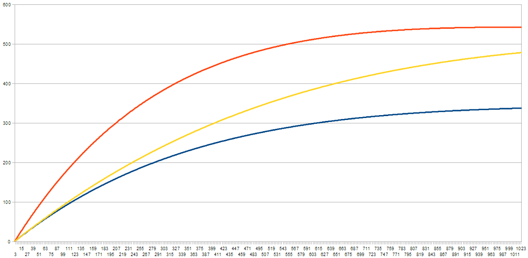
bit of code, you can model the system's progression over time. And from that, you get follower curves like these; with a population of 1,000 and varying follow rates
The blue one at the bottom is for a follow rate of 1 in 10,000, and it has a very steady increase. The top, yellow one has a rate 40 times higher, and has a much quicker increase. The orange one is somewhere in between.


Limitations

But the yellow one reaches a peak, then slowly starts to drop. This is because the number of people who haven't already followed yellow is almost 0 - i.e almost everyone has followed them at least once.


And there in lies the problem. As it turns out, this system will eventually reach a point where S is empty, and the sizes of I and R become constant (a stationary point). This happens when I = (r/u)R, and how fast it happens depends on f.

In other words, for the above curves, since u and r aren't varied they will all stop when I = 250 and R = 750. The only difference is how quickly that happens.

But you could say it's sufficient over relatively short periods of time.


Improvements

First of all, the above model assumes the population (N) is constant - that is, that accounts aren't created or deleted. And obviously this isn't true, so it needs to be included to get a more accurate model.

So we introduce a birth rate, b - how many new accounts are created per unit time, assuming that any variation over time is relatively small. If the changing birth rate is significant and predictable, then it can be easy enough to account for. But for simplicity, we'll assume it's constant.

We also introduce a death rate, and for this we have two possible approaches:
- Either we assume that some proportion (1 in 10,000 or whatever) are deleted in a given time period.
- Or else, we assume a given, relatively fixed, number (say 100 a week) are deleted.

It's a question of whether death rate is constant, or proportion to number of users, and it's a quality of Twitter that you'd have to measure to find out. For simplicity, though, we'll say it's a proportional rate, value d.


The other thing to consider is the effect of the followers you already have - for example, new followers through friends of friends, or through increased exposure as a result of Follow Fridays, retweets, mentions, etc.

Now, as anyone who's used Twitter for a long enough period knows, #FFs don't actually have much effect, almost to the point of being insignificant. But it's still worth including, even if it's given very little 'infective power'.

And this is more like epidemiology, in that the more followers (infectives) you have, the more people there are to 'pass you on' to others. So we introduce a new term,

mI*ln(S) - where ln() is the natural logarithm function. This is important because for a large population, S, (as in the real world) if we didn't take ln(), this term would quickly over-power the rest of the model and follower numbers would grow very large very quickly.

m basically measures the ability of your followers to pass you along, which again is affected by how 'awesome' (or otherwise) you are. But at the same time, if your followers aren't the types of people who RT or FF or whatever, then your awesomeness becomes irrelevant.


Updated Model

So the new model looks something like this,
And as with the previous one, you can write a bit of code to simulate the system, you can play with variables and get an idea of how the system works, what happens when you do such and such, and so on.

Here are some example curves,
The blue one has f at 1 in 1,000 and m as 1 in 10,000, and what you can see is it grows steadily and stays fairly low - it's growth is limited and it essentially flattens out.

The orange one doubles f (keeping everything else the same). And you get the same sort of shape; it just grows faster and levels off higher.

The yellow is the same as blue, but with m doubled. And it falls somewhere in between the previous two - albeit less curved - but doesn't have the same levelling off (within the range of the graph).

Basically, the behavior of this model in most cases goes like this:

- Followers (I) will grow at a rate based, mostly, on the values of f and m.
- It will typically (eventually) reach a point where it's growth slows, almost to the point of not moving for long periods - it becomes pseudo-static - but ultimately it is still increasing.
- The point at which it reaches that pseudo-static state and how high it goes will depend on the variables (f,m,u,r), which is ultimately, relatively unique to each user.

Some other things to consider as well,

- In general, the birth rate is greater than the death rate. But by using a constant birth rate and proportional death rate, you find the population eventually stabilises and becomes constant at N = (b/d). But this is only a problem is the real-world death rate is proportional.
- As far as I know, this model doesn't have any stationary points. But then again, I didn't check. If they do exist, I imagine only the most popular celebrities will experience them. And that's only if the population becomes constant or starts to decline.


In the Real World

So this is still just an approximate model of follower growth. In the real world, you get a lot more 'noise' - one day you might get 3 new followers, but it could turn out they're all spam bots, and over the next week, they disappear one by one. This model essentially averages out that noise.

If you wanted to simulate this behaviour, you can add randomness into the (code) model. But as with the real world, it's ultimately just noise and not really necessary.

So the behaviour of the model may not be as rich as in the real world, but it's 'close enough'.

Other things that aren't accounted for are the fact that variables may change over time. Instead, we assume that their variation is insignificant and can be averaged out. The only time the change would really become significant and worth accounting for is if you suddenly became 'famous' (internet famous counts). But for most people this is not a concern, and more importantly it's not predictable.

The other thing you could add separately is the effect of following people (who don't already follow you). This is typically sporadic. But what you can ultimately do is say, for example, that you follow (on average) n people per week, and that there's an average 50% chance those people will follow you back. And once you've worked that out, you can just factor that value into f.


Usefulness?

If you want a vague idea of how your account's going to grow, this model should suffice. The variables you can get from measurements of your real-life follower growth so far. And from that you can get an idea of when you'll reach your pseudo-static point, and what that point will be (assuming you aren't already there).

But what's perhaps more interesting is if you measure people's personal variables. That way you can assign everyone values for 'attractiveness', 'retention rate', etc. And what you get is a new way to quantify a person's worth, or Twitter quality.


And as a final note, this model doesn't really apply to Facebook since FB doesn't have the follow mechanism, and because you're not getting connections from random people. It would, on the other hand, work for Tumblr, (with possibly some minor adjustments), as well as other sites with a similar follow mechanism.


Oatzy.


[Pro tip: people like to be able to put a number on how much better they are than their friends.]

Flowcharts created with free, online app Lucid Chart

Saturday, January 01, 2011

Life by Numbers: End of Year Report

General

Age: 21
DOB: 18/01/89
Height: 6ft 2.5
Weight: 11st 10
BMI: 20.8


Lifestyle & Money


Average night's sleep: 8hrs 34
Typically asleep between 2:30am and 11am
Minimum sleep duration: 5.5hrs
Maximum: 11hrs

Job interviews: 1
Jobs: 0
Job Seeker's Allowance received: £1,660.88

Major expenditures:
Acer Aspire 5542 - £430
HTC Desire - £150 up front (+ £20/month)
Two nights at Hotel 53 (Valentines weekend) - £264

Monthly subscriptions, Jan 2010: £49.99
Current monthly subscriptions: £33.98

Total spend on Amazon.co.uk - £231.77

Overdrawn: 3 times
Maximum: -£17.52

Net change in bank balance*: -£59.24
Net worth as of 31/12/10: £715.87

Dog walks: 1
Visits to the gym: 2
1 new pair of Adidas trainers; Used twice.
1 new pair of Converse, black.


Entertainment

Most listened to artist: Pink Floyd
Most listened to song: Change by Karnivool
Most listened to album: Sound Awake by Karnivool

Books read cover to cover: 4
* Chuck Palahniuk - Survivor
* Chuck Palahniuk - Snuff
* Richard Bach - Illusions
* Neil F. Johnson - Simple Complexity

Books started but not finished: 7
Graphic novels read: ~12

Films seen at the cinema: 3
* The Lovely Bones
* Inception
* Scott Pilgrim vs The World

2010 released films seen: 6

Films rented (LoveFilm): 10

Words written for NaNoWriMo: 28,369
Percent to target: 56.7%

Games bought: 2
* Pokémon SoulSilver
* Professor Layton and the Lost Future


Food and Drink

Average cups of tea per day: 3.35
Percent of all drinks that are tea: 53.5%

Percent of all drinks that are alcoholic: 19.7%
Approximate average units per week: 13*

Favourite alcoholic drink: Whiskey (bourbon)
As percent of all alcoholic drinks: 52%

Second most drank: Wine (21%)

Most frequently eaten animals*:
1 - Cow
2 - Chicken
3 - Pig

Favourite meals:
1 - Ham and Cheese Sandwich (4.25 a week)
2 - Bolognese (1 every 8 days)
3 - Mixed Kebab & Chips (1 every ~9 days)

Favourite Snack: Ice Cream
Average bowls per week: 2.65

Beer festivals: 1
Visits to Cadbury Land: 1


Travel & FourSquare

Current Mayorships: 16
Badges: 15

Percent of days checked-in on: 58.7%
Average number of 'days out' per week: 4
Average check-ins per 'day out' - 3.68

Most frequently visited venue: Costa Coffee (Parkgate)
Check-ins per week: 1.6

Most frequently visited franchise: Costa Coffee
Days out that include visiting a Costa: ~67%

Check-in locations (via 4mapper):
Local (red spot=home)


Long distance train journeys: 7
4 x Birmingham
2 x York
1 x Loughborough
Total cost: £127.25

Vintage train events visited: 2
Vintage train magazines appeared in*: several, unwittingly


Twitter

Total tweets (as of 31/12/10): 9091
Days online: 608
Average life-time tweet rate: 15 tweets/day
Average tweet rate over 2010: 30.5 tweets/day
Most tweets in a single day: 93 (on 08/09/10)

Composition of tweets:
34.3% Replies
5.46% RTs
0.35% #FF

Average tweet distribution over 1 day:
New friends*: 28
Total foll/followers (as of 31/12/10): 57/120

Most talked to friends:
@aaangst (3.69)
@PkmnTrainerJ (3.04)
@SallyBembridge (3.01)
@Shinelikestars_ (2.26)
@Aerliss (1)

Replies to the above 5 made up 27% of all my tweets; 79% of all replies.

Tweets retweeted: ~1 in 26
Equivalent RTs per day: 1.17


Notes

* Net change doesn't take into account cash and savings. Net worth does.
* based on an assumed average of 1.5 units per serving. Recomended maximum intake: 21 units/week.
* based on which animal the main meat constituent (of a meal) came from.
* no, I don't know which publications precisely.
* 'friends' here defined as a mutual follow. Though I would consider most of them friends, to varying degrees.


You can compare these numbers with those from August 31st here.

Further stats on individual websites below. Due to various reasons there are limits on what data I actually have. So it's worth pointing out that following websites only cover the last -% of the year,

Daytum - 80%
FourSquare - 74%
Twitter (Twoolr) - 66%

Though the interesting thing about Twitter is that while the data I've got only covers 40% of my total time on Twitter, it covers 81% of my total tweets!

Secondly, some of the details (datum in particular) is loose estimates - things are measured in 'serving' and imprecisely at that. FourSquare only logs places where I can and have checked-in - people's houses, or places not on FourSquare aren't logged.

There are also things I didn't/couldn't track, which I might consider in future. For example local trains and buses I don't get tickets for because I travel for free. DVDs, I can remember which I've bought this year, and films I can't remember precisely what I've seen. Cash transactions I didn't track. And so on.

The question is ultimately whether I care enough about having the record to bother to put in the extra effort. That remains to be seen. It's a very fine balance between detail and sanity.


Oatzy.